Q51568 Write a note on Additional and Extended Relational Algebra Operations.

Answer:

This language is used to manipulate the data in the data model. This languages uses a set of operators that are applied on two relations (input) and produces a new relation (output).

Using the different operators-defined by the relational algebra, queries are built and applied on the relations.

1.   Relational Algebra Expression

Consists of operations when applied results into a new relation representing the different requests.

Unary Operations

Operations which operates on only one relation.

Binary Operations

Operations which operate on two relations.

To understand the concepts of relation algebra and relational calculus, the following database “COMPANY” will be used throughout the unit.

COMPANY database consist of five tables with attribute set as shown. EMPLOYEE (E name, Bid, B date, Address, Sex, Salary, D No, Phone number, age)

DEPARTMENT (D Name, D No. Manager-id)

DEPT _LOCATION (DNo. Dlocation)

PROJECT (PName, PNumber. PLocation, DNo, Bid)

DEPENDENT (e id, Dep-Name. Sex, relationship)

The underlined attributes represent the primary key for the respective tables.

A compute view of “COMPANY” Database:

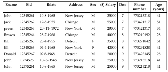
The different operations of relational algebra are:

Select ( σ)

The symbol for the select operation is  σ. This operation is used to select particular rows from the two relations, which satisfy the given condition.

The syntax for select operations (table name) <condition>

Example:

1.   σ (DEPENDENT) Sex = F

This can be read as “select from table DEPENDENT where Sex = F”. The following table will be displayed.

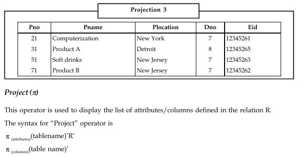
Example: To display project No, DNo from relation PROJECT,

we can write:

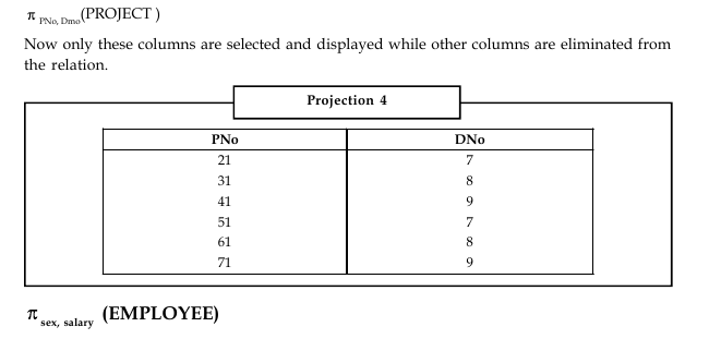
This query will display the columns sex and salary from employee. However, it must be noted that the duplicate values are not repeated in the new relation. Only unique topples are listed. This elimination of duplicate values is called as duplicate elimination and hence reduces redundancy. The following relations will be displayed.

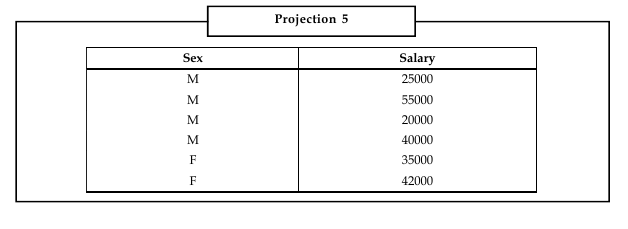
The number of columns returned by the project operator is always equal to or less than the number of columns in the original relation.

To manipulate the data stored in a table we can combine the two operators discussed so far.

Example: If we want to display the emp-id, emp-name, Birthdate, salary of all the employees whose age is greater 30, we can write the expression as,

This will return the following relation:

Selection and projection operators are unary operators, they can be applied to only single relation.

2.        Set Operation of Relational Algebra

The different operators of relational algebra are as follows:

Union (∪)

When applied on two relations, it returns all the rows which are either present in first relation or second relation or in both the relations. It does not return the rows which has the same tuple values – repeating rows. All the rows returned by this operator are unique. One of the constraints of union operator is that both the relations must be union-compatible, i.e., both the relations must have the same number of columns and also these columns must have the same domain (type of data being stored in each column).

If A and B are two relations and are union compatible then union of these two relations is expressed as:

A ∪ B     A → B returns uniquely all the tuples of A and B.

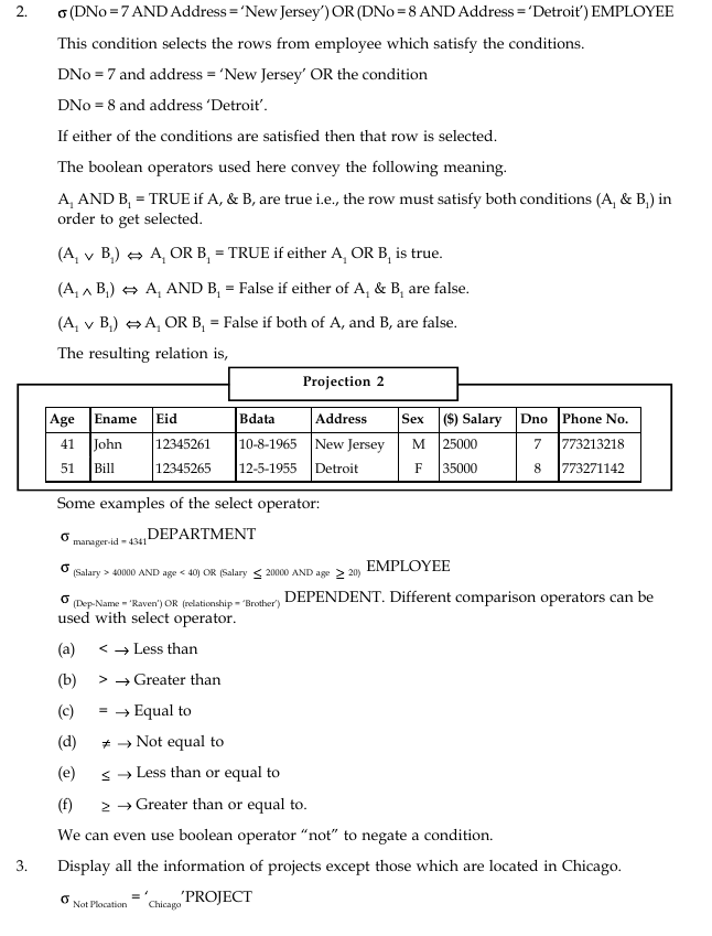
Example: If   we   apply   union   operator   on   EMPLOYEE   relation   and   projection 2 relation then we will get the original employee relation with-only unique tuples. To understand this, consider a simple student1 and student2 relation which represent juniors and seniors.

Roll No	Class	Name
2101	VIII	Ravi
2102	VII	Kumar
2103	VI	Sheena

Roll No	Class	Name
3101	IX	Sodir
3102	X	Dhani
3103	XI	Rahul

Roll No	Class	Name
2101	VIII	Ravi
2102	VII	Kumar
2103	VI	Sheena
3101	IX	Sodir
3102	X	Dhani
3103	XI	Rahul

Intersection (⋂)

When applied on two relations, A and B, it (A⋂B) returns all the rows which are common to both the relations. Most importantly, this operator can be applied to only those relations that are union compatible.

Example: If we apply intersection operator (⋂) to S₁ and S₂ (above relations) then the result will be an empty relation as nothing is common between the two.

S₁⋂ S₂ = ~ empty relation.

If we apply intersection operator (n) on employee relation and projection 2 the resulting relation will be similar to projection 2 relation as it has only two tuples in common.

Set-difference (Minus ‘–’)

This operator is also called “Minus” operator. If A and B are two relations and are union compatible then (A – B) will return all the rows which are in A bit not in B. Consider, this operator is applied to employee and projection 2 relations, then the resulting relation is,

Ename	Eid	Bdate	Address	Sex	($) Salary	Dno	Phone No.	Age (years)
Jack	12345262	12-5-1955	Chcago	M	55000	7	773313218	51
John	12345261	10-8-1965	New	M	25000	8	773213218	41
			Jersey
Green	12345263	20- 11-1 972	New York	M	20000	7	773421317	34
Brown	12345264	28-7-1968	Chicago	M	40000	8	773210192	28
Jill	12345266	04-4-1965	New York	F	42000	8	773291828	41
Donald	12345267	02-8-1968	Detroit	M	20000	9	773423175	28
John	12375261	10-8-1965	New	M	25000	9	773213218	41
			Jersey

Cross Product (*)

This operator returns all the tuples of relation A plus all the tuples of relation B. Cross product is denoted as, A * B – returns the Cartesian product of two relation. The resulting relation will be much bigger in size than the two relations.

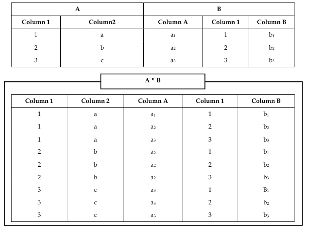
This operator is used to rename the relation or attributes or both. The syntax for this operator is ρ (A (old name  → ρ new name), B)

B is the old relation which being renamed as ‘A’. The list which contains the new names for attributes is called as renaming list.

i.e., old name → rename. This list is used to rename the attributes.

Example: If we want to rename the relation DEPT-LOCATION to DLOCATION and also the attributes DNo to D-number and DLocation to D_L then we can write this as:

ρ (DLocation (DNo → D_number, DLocation → D_L) DEPT_LOCATION)

Its not compulsory to rename both relations and attributes. It depends on the user and this operator simplifies the presentation of different relations (with different names and different attributes). The exclusion of both the relation names and attribute names is meaningless.

3.     Joins

Joins are used to combine the information of two relations which have at least one field in common. It is one of the most important operators of RDBMS. In simple words, a join operation can be defined as a cartesian product followed by selection or projection operators. The different forms of join operators are,

1. Conditional join
2. Equi-join
3. Natural join
4. Outer join.

Conditional Join

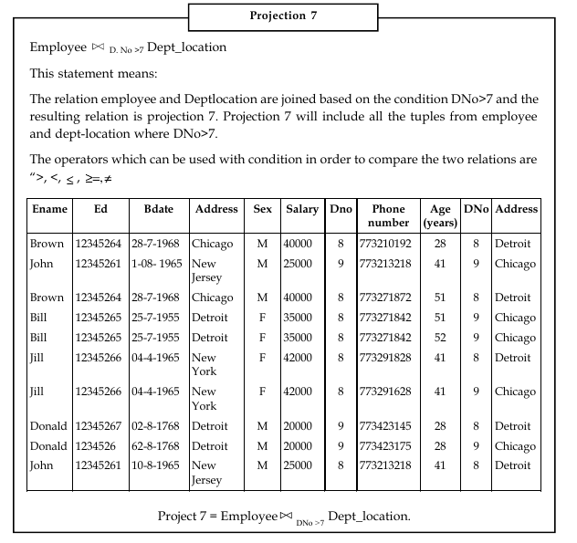
This join returns a relation that includes a set of rows from the cartesian product of two relations A and B such that each row satisfies a given condition C. This can be denoted as,

i.e., join A and B based on same condition. This join is equivalent to performing a cartesian product on two relations followed by a selection operator. Thus,

The application of conditional join on relations employee and Dept_location results into a new relation whose degree is 11.

Degree

The degree of a relation is equal to the number of fields (columns). Consider the equation

Equi-join

Equi-join is same as conditional join, the only difference being only equity ‘=’ operator is used to join the two relations.

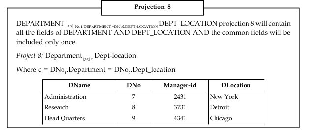
Example: We may join DEPARTMENT and DEPTJLOCATION relation with the condition that

DNo₁. Department = DNo₂.Dept_location.

Where DNo₁ and DNo₂ are two instances of respective relations. This condition indicates – join the tuples where DNo₁ = DNo₂. The degree of resulting relation will be the sum of degrees of two relation minus the number of fields they have in common. More precisely,

The degree of relation A is x

The degree of relation B is y and the number of common fields is z

Then degree of resulting relation = x + y – z.

Natural Join

This is the default join operation i.e., no condition is specified. Natural join is equivalent to cartesian product. If two relations have a common field then the application of natural join is equivalent to equi join and if no field is common then the natural join is cartesian product of the two relations.

We can denote the operation as,

If we apply natural join operation as Departments and dept-location then the result will be same as projection 8 as they have only DNo field in common.

Outer Joins

This is a special case “join” operator which considers the NULL values. Generally a ‘join’ operation performs the cross product of two tables and applies certain join conditions. Then it selects those rows from the cross product that satisfies the given condition. But with outer joins, DBMS allows us to select those rows which are common (satisfies the given) and even those rows that do not satisfy the given condition. To understand this, consider simple instances of project and department table as shown.

If we perform join operation on these two tables.

SELECT *.D₁ * .P₁

FROM Department D₁, Project P₁

WHERE D₁ .PNo = P₁ .PNo

The result of this statement is as follows:

Dept_Mid	DNo	PNo	(PNo)	Pname
101	2	11	11	A
97	5	22	22	B

This table shows the simple join operation of two tables – only those rows are selected that satisfied the condition. However, if we want to include those rows that do not satisfy the condition, then we can use the concept of Outer joins.

There are three types of outer joins namely: (1) Left Outer Join, (2) Right Outer Join and (3) Full Outer Join.

1. Left Outer Join: Left outer join lists all those rows which are common to both the tables and also all those unmatched rows of the table which is specified at the left hand side.

Example: The application of left outer join will result is the following table.

SELECT * .D_l, * .P₁

FROM Department D₁, LEFT OUTER JOIN Project P₁

WHERE D_l.PNo = P_l.PNo.

Result

Dept_Mid	DNo	(PNo)	(PNo)	Pname
101	2	11	11	A
97	5	22	22	B
120	4	33	NULL	NULL

So, the left outer join resulted in a relation that have common rows from both the tables and also the row which does not have match in the other table. The values of the attributes corresponding to second table are NULL values.

2. Right Outer Join: Right outer join is same as the left outer join but the only difference is

the unmatched rows of second table (specified on the right hand side) are listed along with the common rows of both the tables.

SELECT *.D₁, *.P₁

FROM Department D1 RIGHT OUTER JOIN Project P1

WHERE D₁ .PNo = P₁ .PNo

Dept-mid	DNo	(PNo)	(PNo)	Pname
NULL	NULL	NULL	44	D
101	2	11	11	A
97	5	22	22	C

The values of attributes for the first table are declared as NULL.

3. Full Outer Join: This is same as the right outer join and left outer join but only difference is unmatched rows of both tables are listed along with the common tows of the tables.

SELECT *.D₁ * .P₁

FROM Department D₁, FULLOUTER JOIN Project P₁

WHERE D₁.PNo = P₁.PNo

The following table shows the result

Dept_Mid	DNo	PNo	(PNo)	Pname
101	2	11	11	A
97	5	22	22	B
120	4	33	NULL	NULL
NULL	NULL	NULL	44	D

In this relation as you can see all the matched and unmatched columns of both the tables are displayed, the values for the unmatched attributes are entered as NULL.

Division

To understand the concept of division operator consider a simple example of two relations with attributes customer name, product id.

1. Customer (Customer name, product id)
2. Product (Product id)

The result of applying the division operator on relations customer and product is shown in the “Result” relation.

A division operator returns a relation (result). That is a collection of rows from first relation (customer) such that for every value in second relation (product). There exists a pair (customer name, product id) in the first relation (customer).

Customer Customer name Ravi Kumar Girish Sharma Rahul

Product id 1021321 30991231 2310219 1021321 30991231

Product Product id 1021321 30991231

Result = customer/product Customer name Ravi Sharma Kumar Rahul

The division operation is reverse of cartesian product. We can note that

(Customer/product id) = (customer name) * (product id)

Customer = Result * Product

A binary relationship sets is a relationship between only two entities.